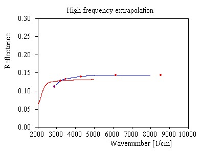
Here we continue to practise extrapolation techniques. From the 'Measurement and extrapolations' window open the 'High frequency extrapolation' and see this initial graph:
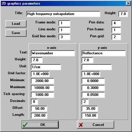
Here we have to do some more adjustments. First of all we have to change the graphics settings in order to display the spectrum also below 2000 1/cm which is the high frequency extrapolation threshold. Actually, it would be a good idea for you to follow the graphics course in order to handle the control of graphics in software of M.Theiss Hard- and Software. With mouse and keyboard commands you can move and zoom quite elegantly. Alternatively, you can set all parameters in a quite large dialog that opens with the command Graphics|Edit plot parameters:
Here we just want to change the Minimum of the x-axis from the current setting 2000 to 1000. You should also change the 'Tick spacing' for the x-axis to 2000. Having done so, leave the dialog with OK:
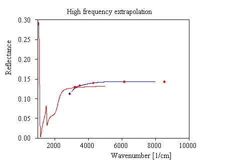
Now use the Range command and set the spectral range of the blue curve to 1800 ... 8000 1/cm with 501 points. Then start with a new set of points with the command Points|Reset points. Now the window shows the following graph:
Now play the 'point move game' a little. For high frequencies the reflectance should approach smoothly a constant level. We could try something like this for the moment:
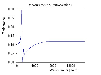
Of course, it is not easy to guess at what level the reflectance curve should be at infinity. Fortunately, we will soon get some help from an inspection of the response function. Close the 'High frequency extrapolation window' for the moment and go back to the 'Measurement and extrapolations' window. Press Update and find the following smooth extrapolated reflectance spectrum:
In case you could not follow this example up to this point you can load the present configuration (using the command File|Open in the main window) from the file step3.kkr that is distributed with the program.