Now you can close the window entitled 'Measured reflectance' and go back to the window called 'Measured reflectance and extrapolations' that is opened from the main window using the command Objects|Input spectrum: Intensity reflectance.
Activate the Update command and see that new measured data have been loaded:
First we set new extrapolation thresholds. Open the corresponding dialog by Objects|Extrapolation thresholds and set the values to 800 and 2000 1/cm, respectively:
Press Update and observe that the new settings take affect:
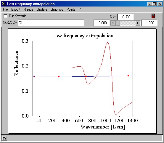
Now let's start with the low frequency extrapolation. Open its window by Objects|Low frequency extrapolation and find the following current situation:
The red curve shows the measured data which are displayed to serve as a guide for the extrapolated curve. The blue line shows the extrapolation which is obtained by a cubic spline interpolation between the 4 red definition points. The latter can be moved with the mouse. While you move the points the interpolated curve is updated continuously - you can immediately see what happens to the data.
Note that the range of the interpolated curve (which can be changed using the Range command) starts at 0 and ends significantly above the extrapolation threshold at 800 1/cm. In addition, it is also very helpful for controlling the spline interpolation that the point at the left end and that to the right are below (and above, respectively) the range of the blue curve.
The goal of the extrapolation is the following: The curve should represent the halfspace reflectance that the material would show if we could measure it. In particular, at the threshold to the measured data (800 1/cm) there must be no jump - a continuous transition of the reflectance data is required. Also the slope should be equal at the threshold. At zero frequency the slope should vanish for physical reasons.
Now let's practise a little and move the four points in order to meet the requirements given above. After a while the situation could look like this:
You could consider this as a reasonable first approach. However, it would be useful for more complicated cases to learn how you can increase the number of definition points of the spline interpolation. If you want to add points you must be very careful with mouse clicks. Activate the menu item Points|Add point and click once at 1000 1/cm in the vicinity of the already existing blue curve. This will create a new definition point. Every click will create a new point, and you should immediately go back to the 'move mode' by the command Points|Move point. Now you can move the new point to the desired position:
If you created too many points you can switch to the 'delete mode' by Points|Delete point and click at an existing point. After the delete operation you should not forget to re-activate the 'move mode' by the Points|Move point command.
If two definition points come too close to each other the spline interpolation may get huge amplitudes. If you are not able to 'repair the curve' you can re-start your work with three definition points which just cover the spectral range of the spline curve. The command for this emergency operation is Points|Reset points.
In the next step we will learn more about setting extrapolations. Close the 'Low frequency extrapolation' window and go back to the 'Measurement and extrapolations' window. Press Update and convince yourself that the extrapolation at the left end of the spectral range looks good now:
In case you could not follow this example up to this point you can load the present configuration (using the command File|Open in the main window) from the file step2.kkr that is distributed with the program.
Extrapolation by a user-defined formula
As alternative to the spline interpolation you can define the extrapolation (or a part of it) by a user-defined function. Check the Use formula checkbox in the upper left corner of the window to do so. In the field to the right of the label Y(X,C1)= you can enter a user-defined formula. The formula must be entered according to the rules in the Data Factory manual. In the formula you can refer to the wavenumber by the symbol X, and to a constant called C1. The value of the constant C1 is displayed in the upper right corner of the window. Below that value there is a slider in between two fields. The slider can be used to scan a range of C1 values which can be useful to adjust the formula to make a continuous transition between extrapolated and measured data. The field to the left of the slider gives the minimum of the 'slider range' whereas the number to the right defines the maximum. While you move the slider, the value of C1, the formula and the graph are updated.
You can specify the wavenumber range where you want to use the formula. This can be used to work with combinations of the formula and the graphical spline definition. The spline data are used in the whole range of the extrapolation curve (i.e. the range that is defined using the Range command) except for the 'formula range'. Here the data computed according to the formula replace the spline data.